Structural Break Test
Coypright: Ralf Elsas, 03/13/2022
Table of Contents
1 Motivation
2 Simulation Parameters
3 Simulation of returns
4 Plot one return time-series
5 Illustrate isolationForest for detecting outliers
5.1 Analyse outliers with structural break present
5.2 Analyse without structural break
6 Measuring time clustering
7 Histogram: Comparison of time correlation
8 Quality of Structural Break Test with bootstrapping and Monte Carlo simulation
9 Conclusions
1 Motivation
Event studies are a statistical/econometric tool to measure the stock price reaction to new, relevant and surprising information. In Single-Firm/Single-Event (SFSE)-studies, testing for statistically significant event period returns is challenging, as inference can only be based on the time-series of returns for the stock (or, more general, the security) under examination.
Elsas/Schoch (2022) show that in this setting estimation is severely biased when calibration and event period occur in different volatility regimes. But changes in volatility regimes are a frequent phenomenon.The most extreme examples are the subprime crisis in 2008/09, or the Corona-fever period in March 2020. However, from 2005 to 2021 the market volatility (measured e.g. by the VIX or the VDAX) changed 15 times by at least one standard devation. Due to the occurence of additional idiosyncratic shocks, changing volatility regimes will be of even greater relevance for single firms, which are at the heart of our analysis.
This script illustrates the statistical characteristics of the unique specification test for such structural breaks developed in the paper by Elsas/Schoch (2022). The focus is on two statistical characteristics:
- The Type-I error of a statistical test provides the relative frequency with which the test rejects a null hypothesis, if the hypothesis is actually true. In the structural break setting, we use simulated returns and test, how often the specification test indicates the presence of a structural break if in fact there is none. In a well specified setting, and using a 5% significance level, this should happen in 5 out of 100 cases.
- The power of a statistical test provides the relative frequency with which the test rejects the null hypothesis if the hypothesis is actually wrong. In the structural break setting, we test how often the specification test indicates the presence of a structural break if in fact there is one.
The desirable outcome of such an analylsis is that the statistical test has the expected Type-I-error (i.e. 5% rejection rate with a 5% significance level) if there is no structural break, and conditional on that a high probability to detect structural breaks if these are prevalent (i.e. rejecting a false null hypothesis with high probability).
This illustrative script uses Monte Carlo simulations of abnormal stock returns with realistic characteristics in three different volatility regimes: low (‚“normal“), medium, and high („crisis“). An abnormal return is the realized stock return on a trading day minus its expected value for that day, which is the central „unit“ of measurement in event studies.
2 Simulation Parameters
The parameters for the GARCH(1,1)-stochastic process used to simulate abnormal returns is calibrated on U.S. companies who were constituents of the DJI index. The scenario with the highest volatility was estimated during the subprime crisis of the years 2008/09, where the capital market was in turmoil after the default of Lehman Brothers on September 15, 2008.
anteil =0.3; % fraction of obs in different first regime (not event period)
vola = 0.4; % base volatility of HIGH regime
cLow = 0.0000357; % constant for GARCH (low regime)
cMedium = 0.0000744; % constant for GARCH (med regime)
cHigh = 0.0000635; % constant for GARCH (high regime)
anteil = 0.2; % first period fraction when strucutural break
nSim = 100;
simObs = 252;
3 Simulation of returns
Simulatíon of the data. The GARCH(1,1) process has t-distributed error terms to model the (relative to a normal distribution) high frequency of tail returns in the empirical data.
mdlLow=garch(‚Constant‘,cLow,‚GARCH‘,0.5,‚ARCH‘,0.1,‚Distribution‘,…
struct(‚Name‘,‚t‘,‚DoF‘,5)); % sigma p.a.= 15%
mdlMedium=garch(‚Constant‘,cMedium,‚GARCH‘,0.6,‚ARCH‘,0.1,‚Distribution‘,…
struct(‚Name‘,‚t‘,‚DoF‘,5)); % sigma p.a.= 25%
mdlHigh=garch(‚Constant‘,cHigh,‚GARCH‘,0.8,‚ARCH‘,0.1,‚Distribution‘,…
struct(‚Name‘,‚t‘,‚DoF‘,5)); % sigma p.a.= 40%
[~,simData]=simulate(mdlLow,simObs,‚NumPaths‘,nSim);
[~,simDataM]=simulate(mdlMedium,simObs,‚NumPaths‘,nSim);
[~,simDataH]=simulate(mdlHigh,simObs,‚NumPaths‘,nSim);
% simulate and store results
breakFrac=anteil;
breakPoint=floor(size(simData,1)*breakFrac);
% simData = simDataH;
simDataBreak=[simData(1:breakPoint,:);simDataH(breakPoint+1:end,:)];
simDataBreakM=[simDataM(1:breakPoint,:);simDataH(breakPoint+1:end,:)];
simDataBreakL=[simData(1:breakPoint,:);simDataM(breakPoint+1:end,:)];
% make parameters table
tRes = table;
low = [0.3.*vola, cLow,0.5,0.1,5];
medium = [0.6.*vola, cMedium,0.6,0.1,5];
high = [vola,cHigh,0.8,0.1,5];
tRes = table(low‘,medium‘,high‘);
tRes.Properties.RowNames = {‚Unconditional Volatility‘; ‚Constant‘;…
‚GARCH‘; ‚ARCH‘;‚t-Degrees of Freedom‘};
tRes.Properties.VariableNames = {‚Low‘,‚Medium‘,‚High‘};
tRes
4 Plot one return time-series
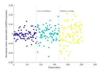
The following graph illustrates the return distributions in the low, medium, and high scenarios using one randomly selected simulated return series. As can be seen, detecting structural breaks is not trivial as extreme returns occur in all scenarios.
werSingleSeries=randi(100);
x1 = [1:252]‘;
y1 = [simData(1:84,werSingleSeries);simDataM(85:167,werSingleSeries);…
simDataH(168:252,werSingleSeries)]; % take low2high, random
c = [repmat(1,1,84),repmat(8,1,84),repmat(15,1,84)];
figure(’name‘,„Example of Simulated Returns“)
p1 = scatter([1:252],y1,[],c,„filled“);
ylabel(‚Simulated return observations (GARCH-process)‘);
xlabel(‚Observation‘);
vLineAnnotation(84,‚Low to Medium‘);
vLineAnnotation(168,‚Medium to High‘);
5 Illustrate isolationForest for detecting outliers
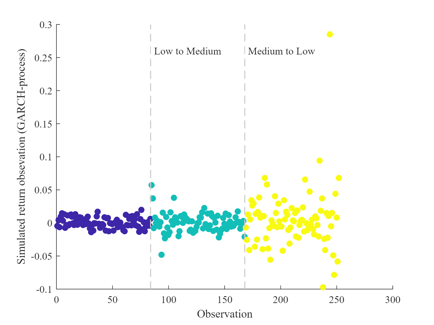
We use the isolationForest algorithm to detect outliers in the return series and construct a statistical test on these outliers to test for the incidence of a structural break in the return volatility.
The code analyzes the simulated return series with (showing a change from low to high volatility) and without structural break (medium volatility)
5.1 Analyse outliers with structural break present
[nObs nSim]=size(simDataBreak);
% parameters for iForest (default)
% NumTree = 100; % number of isolation trees
% NumSub = 256; % subsample size
% NumDim = 1; % do not perform dimension sampling
ScoresRetWith=cell(1,nSim);
werOutlierWith=cell(1,nSim);
anteilWith=nan(nSim,1);
parfor ii=1:nSim
X=simDataBreak(:,ii);
[Mdl,tf,scores]=iforest(X,‚ContaminationFraction‘,0.2);
ScoresRetWith{ii}=log(scores)/2; % standardized scores
end
5.2 Analyse without structural break
ScoresRetWithout=cell(1,nSim);
werOutlierWithout=cell(1,nSim);
anteilWithout=nan(nSim,1);
parfor ii=1:nSim
X=simDataM(:,ii);
[Mdl,tf,scores]=iforest(X,‚ContaminationFraction‘,0.2);
ScoresRetWithout{ii}=scores;
end
6 Measuring time clustering
Our specification test for structural breaks is based on the simple idea that in the case of a regime change, the observation period is divided into (at least) two time periods, where extreme returns occur more frequently in the phase with higher volatility. These relative outlier returns (or synonymous „anomalies“) must also occur in a temporally coherent pattern, as they will be clustered in the high volatility period.
In this step of the script, the temporal correlation of the identified outliers is measured. If outliers occur cluster within time, i.e. show a strongly pronounced temporal correlation pattern, this is indicative of a structural break.
korrWith=cellfun(@(x) corr(x,[1:length(x)]‘,‚type‘,‚Spearman‘),…
ScoresRetWith);
display(„The time correlation with a structural break is “ + mean(korrWith));
korrWithout=cellfun(@(x) corr(x,[1:length(x)]‘,‚type‘,‚Spearman‘),…
ScoresRetWithout);
display(„Time correlation without structural break from LOW to HIGH is „…
+ mean(korrWithout));
7 Histogram: Comparison of time correlation
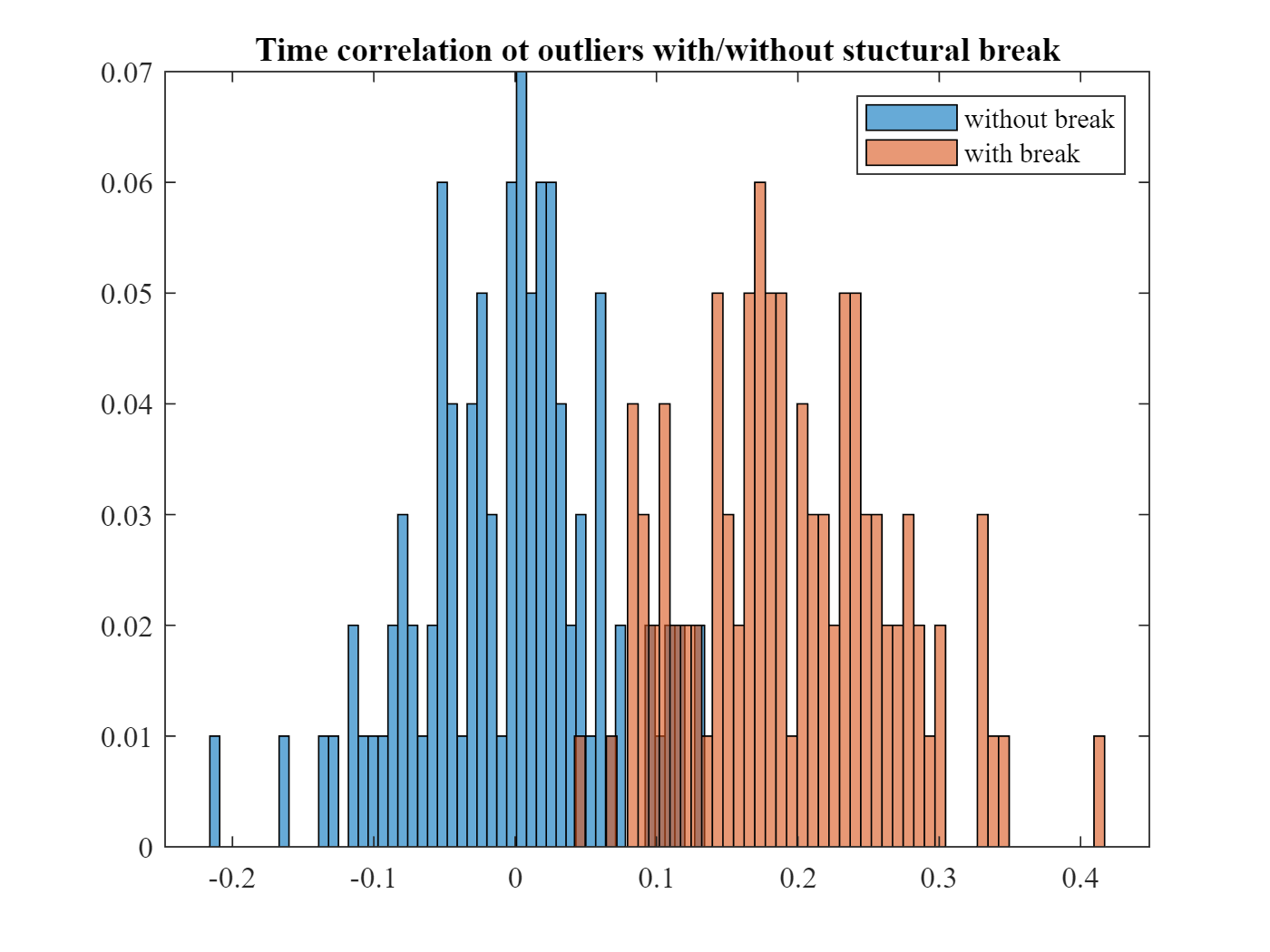
The graph illustrates for the data with and without structural break the distribution of the measured time correlations:
- Without structural break (blue), extreme returns are distributed randomly over time, and correlation with time (clustering) is centered at zero.
- With a structural break (orange), extreme returns occur mostly in one out of two sub-periods, so that there is high time clustering, and correlation with time is systematically shifted away from zero.
figure(4)
histogram(korrWithout,50,‚Normalization‘,‚probability‘)
hold on
histogram(korrWith,50,‚Normalization‘,‚probability‘)
hold off
legend(‚without break‘,‚with break‘)
title(„Time correlation ot outliers with/without stuctural break“);
8 Quality of Structural Break Test with bootstrapping and Monte Carlo simulation
In the final step of the structural break test, each time-series of outliers and the rank correlation coeffcient with time will be bootstrapped. If the rank correlation is different from zero, the test indicates a structural break. We only use 100 simulation runs here, please see the paper for an extensive analysis.
The following code analyzes statistical size and power of the structural break test in four scenarios:
- no structural break (i.e. a test for the size of the test)
- structural break from low to medium volatility (power test)
- structucal break from medium to high volatility (power test)
- structural break from low to high volatility (power test)
resSim=cell(4,1);
tic
for jj=1:4
if jj==1
data=simData; % no break
elseif jj==2
data=simDataBreakL; % low2medium
elseif jj==3
data=simDataBreakM; % med2high
elseif jj==4
data=simDataBreak; % low2high
end
temp = simResBreakNew(data,’nSim‘,nSim,’nBoot‘,100);
resSim{jj,1} = temp.avgBreak;
end
toc
% make result table
S = repmat(nSim,4,1);
expAnteil = [„size test, should be close to 0.05“,…
„power test, higher is better“,…
„power test, higher is better“,,,,
„power test, higher is better“]‘;
powerRes = resSim;
tResSim = table(S,expAnteil,vertcat(powerRes{:}));
tResSim.Properties.RowNames = {’no break‘;‚ low2medium‘; …
‚medium2high‘;‚low2high‘};
tResSim.Properties.VariableNames = [„S=“+nSim,„Expected“,…
‚Sim-Rejection „no break“‚];
tResSim
9 Conclusions
In our paper, we devise a statistical test for a structural break in the volatility of daily abnormal returns using the isolation forest machine learning algorithm for outlier detection. The proceeding for this test is illustrated in this script.
Overall, we believe the structural break test is in statistical terms well specified in the absence of structural breaks and powerful to detect structural breaks even if only approximately 20% of the calibration period’s returns are subject to a different volatility regime and if the time-series is short. The test is – to the best of our knowledge – unique to the academic literature.