Machine Learning for Earnings Forecasts
(by Ralf Elsas, LMU Munich, Germany, 02/19/2024, updated on 03/01/2024 to correct for errors in data preparation)
1 Overview
Earnings predictions by analysts receive a lot of attention in capital markets, e.g. guiding investors regarding the expected future performance of companies. The German security markets supervisory authority (BaFin) recently even designated analysts’ predictions as their regulatory measure for capital market expectations on firms’ earnings, thereby constituting a regulatory benchmark for companies how to (ex-ante) judge the mandatory and timely disclosure of material nonpublic information according to EU’s Market Abuse Regulation (MAR).
However, reliance on analysts has limitations. Firstly, their estimates may be subject to biases arising from conflicts of interest. Secondly, analyst coverage is limited (and steadily decreasing), particularly outside the US.
In this context, Moritz Scherrmann and I have recently developed a machine learning (ML) framework to predict firms‘ earnings-per-share (EPS) using a recurent neural network (RNN) framework (arxiv). Our ML approach offers several advantages, with some of them being unique also to the academic literature:
- The prediction quality of the RNN’s out-of-sample performance surpasses benchmark models from the academic literature by a wide margin and outperforms analysts’ forecasts for fiscal-year-end earnings predictions.
- The network predicts fiscal-year-end and quarterly EPS. Since quarterly predictions are rarely considered in academic models, this feature is particularly useful for issuers and investors, as quarterly earnings announcements are the most important source of information that determines stock prices (explaining on average some 25% of overall stock returns).
- The model is sparsely parametrized with regard to input data, using at most 20 quarters of accounting information (five items), and market data (five items, like the change in volatilty index and a firm’s market-to-book ratio).
- In addition, we explicitly allow for missing values in the accounting variables and control for the age of each information item relative to the prediction day. This greatly reduces inherent survivorship biases due to data requirements, which is often a drawback of academic models.
The model is trained on a large scale dataset for US firms. Can such a model be applied also to firms in other countries or financial (or accounting) systems? This blog post reports results from an experiment, where I apply the model to German firms, also using input data from a Fintech provider (EODhistoricaldata.com). Therefore, not only is the model applied in a full out-of-sample setting, but it is also challenged by relying on different (and comparatively speaking low-cost) data than during training.
All calculations are done using Matlab R2023b.
2 Model and Data
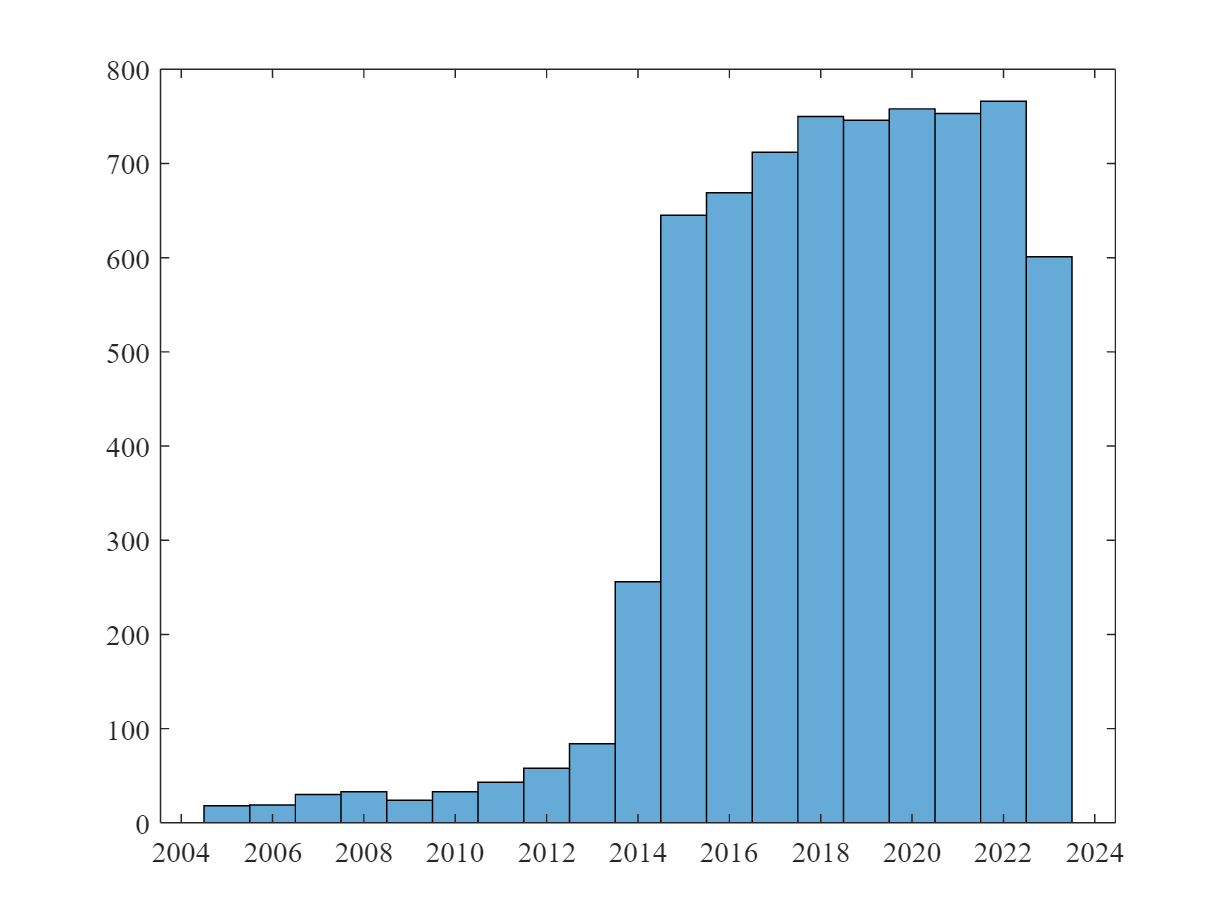
The EPS prediction model uses a simple structure of GRU and feedforward layers and relies (amongst other inputs) on past quarterly EPS to predict both quarter and yearly EPS. For this experiment, the pretrained model is applied to all current (as of 02/15/2024) German exchange-listed companies for which EOD provides accounting information and realized EPS data (284 out of 555 German firms in the EOD database). We predict EPS for each company on the day before the release of the quarterly/annual report. This constitutes a sample of companies over the time period mostly from 2015 until today (see the figure below), overall 6.998 firm-quarter observations. Note that for 48% of these observations no prediction by analysts was available.
3 Prediction Quality (Out-of-Sample)
3.1 Quarterly Predictions
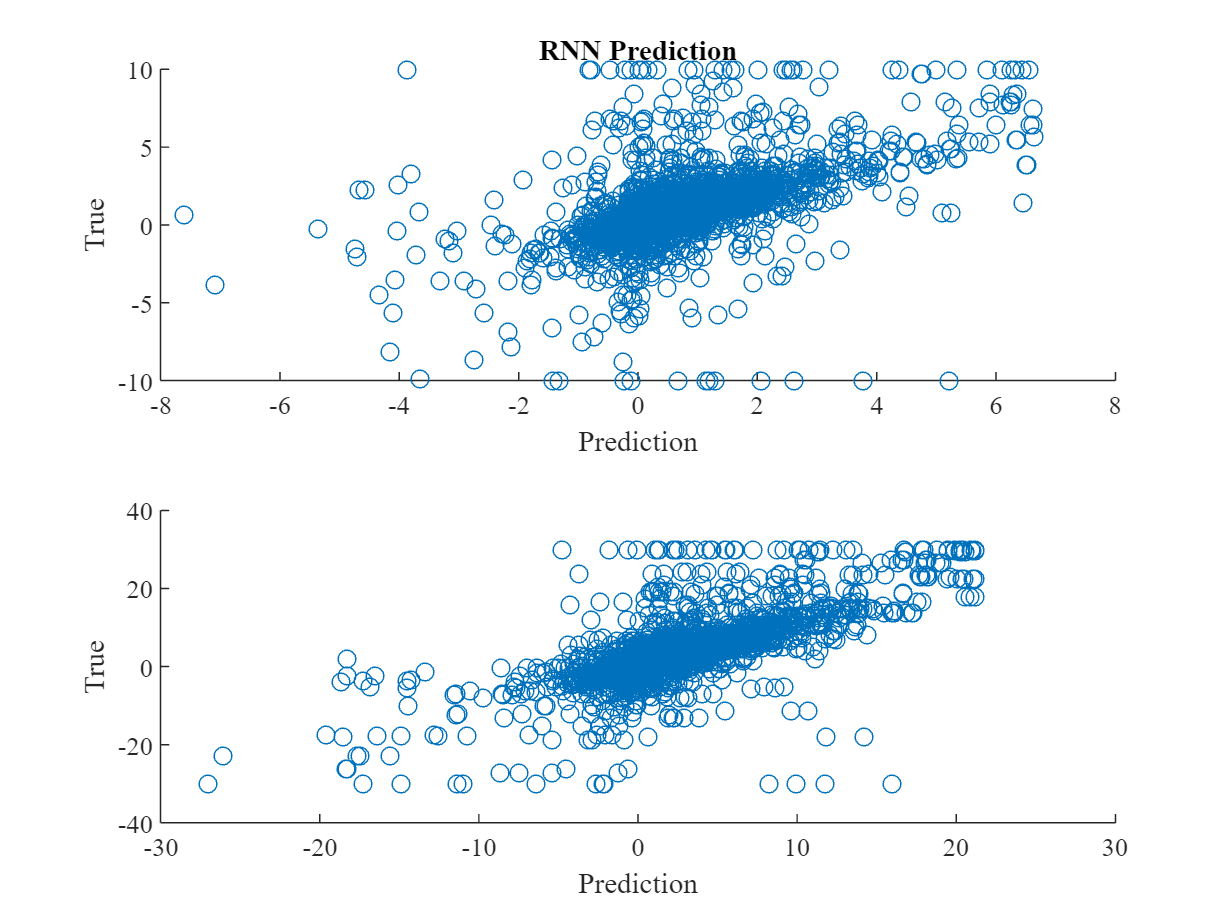
The next graphs show scatter diagrams between RNN and analysts predictions and the subsequently realized quarterly EPS. For a better visusalization and to k´limit the inpact of outliers, we winsorize the data to be in the [€-10, €10] range of earnings per share.
The following table shows results from a simple OLS analysis to test for the relationship between the prediction of the RNN and the actually realized quarterly EPS. It shows that the RNN on average fits the true EPS (with an average of €0.15 underestimation), and explains about 34% of the overall variation in realized quarterly EPS.
OLS results for the analysts are inferior in prediction accuracy compared to RNN. They similarly explain about 34% of the variance of realized quarterly EPS. But on average, analysts‘ consensus estimate (according to EOD) overestimates realized EPS by about 31%, However, most norteworthy is the difference in sample size – 3.651 observations for analyst predictions versus 6.998 observations from the RNN.
A final comparison of RNN predictions on the same dataset as analyst predictions is shown in the next regression. The explained variance slightly increases to 36%, showing that the quality of quarterly RNN predictions are at par with analysts, and EPS accuracy remains Better than those of analysts.
3.2 Yearly Predictions
EOD provides only quarterly EPS forecasts from analysts. Thus, we can only compare RNN predicted yearly EPS to their afterwards realized values. The performance of the yearly EPS predictions from the RNN is even better than for quarterly data. The regession shows about 16% underestimation and an explained EPS variance of 55%. Here, winsorizing was reduced to the [€-30, €30] range per share, as outliers were less severe both for realized and predicted values.
As the last step to test model quality, I calculate the median percentage deviation (MPD) and median absolute percentage deviation (MAPD) for the forecast errors. The median is chosen to be more robust against outliers. Both measures are common choices in the academic literature.
Compared to the results for the US data (on which the model has been trained on), both measures show a deterioriation in model quality, with MPD turning signficantly different from zero and but MAPD being on some level. I leave it to future research to analyze whether an additional fine-tuning of the model on German data could have mitigated this deterioration.
4 Random Walk Benchmark and Data Quality
4.1 Random Walk Benchmark
As a first additional robustness check, the following figure and regression show the performance of a naive benchmark random walk model, simply using the one-year-lagged realized quarterly EPS as the predictor for the upcoming quarterly EPS. In many capital market settings, such a random walk is a strong benchmark for any more structured prediction model, but the results show that this is not the case for EPS predictions. Lagged EPS overestimates EPS significantly by about 77% and only explains about 21% of quarterly EPS variance.
4.2 Data Quality
Fundamental data availability for German companies is way worse compared to their US counterparts. A final question to be addressed is then, by how much data availability and – in particular – missing values affect the prediction quality of the model. It should be reemphasized that one of the key features of our model is that it allows for missing values in the accounting input variables, thereby mitigating too strict data requirements.
The descriptive statistics show that in our sample of 284 German firms, the average fraction of missing values is at about 11%. As there are a maximum of 20 quarters serving as input to the RNN, this corresponds to two missing quarterly observations on average. The 75%-quantile is at 10%, thus about 25% percent of the observations do have missing data, with in the worst case only one observation. However, it should be noted that the sample is already quite selected – out of 555 analyzed German firms, only 296 had information that could be used for prediction in the first place.
The following regression tests whether a higher fraction of missing values has a significant impact on the forecast error of the model (measured as MAPD here).
The regression results show that the fraction of missing values does not affect significanty the model’s forecast errors. Forecast errors are mostly dependent on how much quarterly information about the current fiscal year was already available. This finding illustrates that our model design indeed provides for robustness against missing values in the accounting data input.
5 Conclusion
This blog discusses earnings prediction based on a new approach, relying on a parsomonious neural network which is designed to allow for missing values in the key accounting input variables, and produces quarterly and fiscal-year-end EPS predictions. As a result, using a machine learning based approach for earnings prediction is robust and powerful:
- The model is applied to data from a different country (Germany), where firms are subject to IFRS accounting standards instead of US-GAAP (as in the US training data). Still, EPS predictions have high quality, being at least on par with analysts‘ forecasts.
- The most important advantage of the ML approach is, however, that one can get reasonable EPS estimates on a quarterly and fiscal-year-end basis also for firms not covered by analysts. In the analyzed sample, analysts‘ forecast are available in only 50% of the cases for which the model could predict EPS.
- The analysis also demonstrates that the neural network can be designed such that the model is parsimonious in terms of data requirements and missing values in accounting input data are allowed, without harming prediction quality (if not too severe to prevent estimation in the first place).